Now, let us look at a dynamical process in a hypothetical environment, a process producing n variants of some outcome. It could for example be an ecosystem, producing a sequence of delicate balances between its constituent species. Let it be given by an equation system
dxj/dt = Xj(xj, t, a, b,...)where x measures the population level of each species, t is time and a, b... are auxiliary parameters, describing factors affecting the overall process. A state of the system is given by the parameters (xj, t, a, b...) of dimensiom n + 1 + the number of auxiliary parameters. The Euclidean space of the same dimension is called the phase space M of the system. If a state is of some duration and resists slight perturbations we may envisage it as being kept in place by low potential, an attractor, representing an energy minimum relative to the immediate environment (in analogy the maxima are termed repellors.). The above full dynamical system (M, X) is often unnecessarily complicated (and in most cases impossible to solve) but it may be parametrized by a mapping from M to R, the set of real numbers, e.g. by introducing a real-valued potential function V and letting X = -grad V, where X is the original gradient field. Now V serves to describe the potential keeping states "in place" but also (where relevant) the transitions between different states. (These mappings are not random, but very "chosen", and they may be shrewdly manipulated; I will return to them later on).
Local maxima, minima and inflexion points of any function f are given by its critical points, points where the graph of the function has a horizontal tangent. With the number of variables these points become more and more complex; there will occur more complicated attractors: a.o. saddles and troughs. The critical points are obtained by putting the first derivative of the function = 0. If the first derivative = 0, and the second derivative is a nondegenerate quadratic form, we say that f has a nondegenerate critical point. Nondegenerate critical points are always isolated. Around such a point, there always exists a local system, where the potential function V (in the above equation: X = -grad V) can be expressed as a quadratic form. In the twenties the American mathematician Marston Morse pointed out, that the critical points of the "complete" dynamical system belonged to either of two main types: Morse-critical, structurally stable ("generic") points related to normal action well within the different phases/states, and a more rare category: degenerate, non-structurally stable critical points (points where f'(x) is not transverse to y = 0, i.e. where f'(x) = f''(x) = 0), and these latter points are uniquely related to the transition zones between states. A theorem connects the realm of stable states with areas incorporating Morse-critical points, and the critical, unstable border-zones with degenerate critical points. The unstable zones of state transitions are the "catastrophes" in the terminology of Thom and Zeeman. In the fifties it was shown by among others Thom, that the complete state function can be split up into two components, one major, "Morse" component related to the stable areas, one minor, degenerate component, whose number of variables equals the corank of the function. The behaviour of the overall state function near the degenerate critical point(s) (phase shifts, transitions between states, catastrophes) can be found by studying this second component. The "splitting lemma" has a very central position within the theory: if we have a thousand variables in a function of corank 2 we only need to study a function with 2 variables in order to learn about the behaviour of the function in the vicinity of the degenerate critical point.
This implies: we can leave the complete, incalculable systems of differential equations describing the "interior" qualities of a dynamical system aside and concentrate on e.g. a more manageable gradient function (some quadratic or cubic form, more about this later on), producing the catastrophes. As early as 1971 Thom had outlined this shift away from a purely quantitative (and in most cases: vain) approach to a qualitative approach:
Even if the right hand side of (the system of differential equations: dxj/dt = X(xj, t, etc.)) is given explicitly, it is nevertheless impossible to integrate formally. To get the solution one has to use approximating procedures.How does a small perturbation influence a critical point? We say that f as a critical point is structurally stable if a small perturbation leaves the type (Morse/degenerate) of the critical point unchanged. A minimum remains a minimum - even if its location is moved. This applies only to nondegenerate critical points; if a degenerate point is perturbed "anything" may happen. The notion of structural stability may be extended to functions: f is structurally stable if, for all sufficiently small functions p, the critical points of f and f + p have the same type (f and (f + p) are equivalent, after a suitable translation of the origin). Near a Morse critical point any function is structurally stable. [x2 perturbed by a term kx still has one Morse critical point, but the point is moved; x3 perturbed by kx has no critical points at all for positive k, and two for negative (implying:x3 is structurally unstable as a critical point); x4 perturbed by kx2 has one single Morse minimum, or two minima and one maximum. The higher the degree of n, the worse the behaviour of xn in this respect].
For these two reasons, one has to know to what extent a slight perturbation on the right hand side of the equation system may effect the global behaviour of the solutions. To overcome - at least partially - these difficulties, the mathematician Henri Poincaré introduced in 1881 a radically new approach, the theory of 'Qualitative Dynamics'. Instead of trying to get explicit solutions of the equation system, one aims for a global geometrical picture of the system of trajectories, defined by the field X. If this can be done, one is able to describe qualitatively the asymptotic behaviour of any solution. This is in fact what really matters: in most practical situations, one is interested not in a quantitative result, but in the qualitative outcome of the evolution. Thus, qualitative dynamics, despite the considerable weakening of its program, remains a very useful - although very difficult - theory. (2)
Transversality and structural stability are the topics of Thom's important transversality and isotopy theorems; the first one says that transversality is a stable property, the second one that transverse crossings are themselves stable. These theorems can be extended to families of functions: If f: Rn x Rr-->R is equivalent to any family f + p: Rn x Rr-->R, where p is a sufficiently small family Rn x Rr--> R, then f is structurally stable. There may be individual functions with degenerate critical points in such a family, but these exceptions from the rule are in a sense "checked" by the other family members. Both the Morse and the Splitting lemma can be extended to families of functions. Such families can be obtained e.g. by parametrizing the original function with one or several extra variables. Thom's classification theorem, comes in at this level, it is stated in the wordlist.
So, in a given state function, catastrophe theory separates between two kinds of functions: one "Morse" piece, containing the nondegenerate critical points, and one piece, where the (parametrized) family contains at least one degenerate critical point. The second piece has two sets of variables; the state variables (denoted x, y...) responsible for the critical points, and the control variables or parameters (denoted a, b, c...), capable of stabilizing a degenerate critical point or steering away from it to nondegenerate members of the same function family. Each control parameter can control the degenerate point only in one direction; the more degenerate a singular point is (the number of independent directions equal to the corank), the more control parameters will be needed. The number of control parameters needed to stabilize a degenerate point ("the universal unfolding of the singularity" with the same dimension as the number of control parameters) is called the codimension of the system. With these considerations in mind, keeping close to surveyable, four-dimensional spacetime, Thom defined an "elementary catastrophe theory" (not yet in list) with seven elementary catastrophes, where the number of state variables is one or two: x, y, and the number of control parameters, equal to the codimension, at most four: a, b, c, d. (With five parameters there will be eleven catastrophes). The tool used here is the above mentioned classification theorem, which lists all possible organizing centers (quadratic, cubic forms etc.) in which there are stable unfoldings (by means of control parameters acting on state variables). In this excurse, I will stick to elementary catastrophe theory and the two simplest catastrophes: the fold and the cusp.
Two elementary catastrophes: fold and cusp
1. In the first place the classification theorem points out the simple potential function y = x3 as a candidate for study. It has a degenerate critical point at {0, 0} and is always declining (with minus sign), needing an addition from the outside in order to grow locally. All possible perturbations of this function are essentially of type x3 + x or type x3 - x (more generally x3 + ax); which means that the critical point (y, x = 0) is of codimension one. Fig. 1 shows the universal unfolding of the organizing centre y = x3, the fold: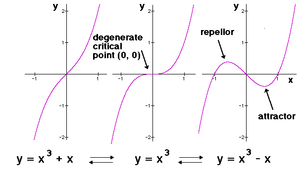
Fig. 1. Universal unfolding: the genesis (from left to right) or destruction (right to left) of an attractor with linear change of the control parameter a from positive to negative values or vice versa. Out of the degenerate critical point {0, 0} of the organizing centre x3, [codimension (f) + 1] critical points are "shaken loose" (unfolded) by the family x3 + ax. As long as a < 0 a stable state of a process remains "caught" or locked in the low potential of the attractor basin.
This catastrophe, says Thom, can be interpreted as "the start of something" or "the end of something", in other words as a "limit", temporal or spatial. In this particular case (and only in this case) the complete graph in internal (x) and external space (y) with the control parameter a running from positive to negative values can be shown in a three-dimensional graph (Fig. 2); it is evident why this catastrophe is called "fold":
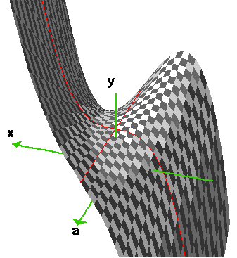
Fig. 2. The fold for -2 < y < 2 and -2 < x < 2. Type y = x3 + x in the fore of the figure, type y = x3 - x takes over from the degenerate critical point x = 0, y = 0 (given by the two derivatives f'(0) = 0, f''(0) = 0).
One point should be stressed already at this stage, it will be repeated again later on. In "Topological models..." (2) Thom remarks on the "informational content" of the degenerate critical point:
This notion of universal unfolding plays a central role in our biological models. To some extent, it replaces the vague and misused term of 'information', so frequently found in the writings of geneticists and molecular biologists. The 'information' symbolized by the degenerate singularity V(x) is 'transcribed', 'decoded' or 'unfolded' into the morphology appearing in the space of external variables which span the universal unfolding family of the singularity V(x). (My emphasis; CP)2. Next let us as organizing centre pick the second potential function pointed out by the classification theorem: y = x4. It has a unique minimum (0, 0), but it is not generic (not yet in list), since nearby potentials can be of a different qualitative type, e.g. they can have two minima. But the two-parameter function x4 + ax2 + bx is generic and contains all possible unfoldings of y = x4. The graph of this function, with four variables: y, x, a, b, can not be shown, the display must be restricted to three dimensions. The obvious way out is to study the derivative f'(x) = 4x3 + 2ax + b for y = 0 and in the proximity of x = 0. It turns out, that this derivative has the qualities of the fold, shown in Fig. 3; the catastrophes are like Chinese boxes, one contained within the next of the hierarchy. The first derivative f'(x) is shown in Fig. 3:
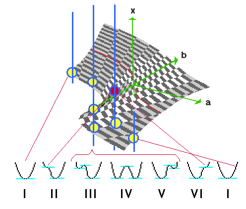
Fig. 3. The derivative of the universal unfolding x4 + ax2 + bx for y = 0. Three major types of vertical intersection with the curve (blue lines) give 1 (upper sheet outside the cusp), 3 (upper sheet + repellor sheet + lower sheet within the cusp) and 1 (lower sheet outside the cusp) Morse-critical points (yellow) and one degenerate critical point (red; f'(x) = f''(x) = 0). When the intersections are moved over the fold they generate five different generic types of potential, these are shown under the graph. The potentials II and VI are connected with the degenerate critical points, where a vertical intersection touches the fold on each side. A state remains caught in the right hand minimum from I to V, in VI the repellor is dissolved (the catastrophe), after which a new state is again caught by a single potential minimum (attractor), but now on the lower sheet.
Finally we look for the position of the degenerate critical points projected on (a,b)-space, this projection has given the catastrophe its name: the "cusp" (Fig. 4). (An arrowhead or a spearhead is a cusp). The edges of the cusp, the bifurcation set, point out the catastrophe zone, above the area between these limits the potential has two Morse minima and one maximum, outside the cusp limits there is one single Morse minimum. With the given configuration (the parameter a perpendicular to the axis of the cusp) a is called the normal factor - since x will increase continuously with a if b < 0, while b is called the splitting factor because the fold surface is split into two sheets if b > 0. If the control axes are instead located on either side of the cusp (A = b + a and B = b - a) A and B are called conflicting factors; A tries to push the result to the upper sheet (attractor), B to the lower sheet of the fold. (Here is an "inlet" for truly external factors; it is well-known how e.g. shadow or excessive light affects the morphogenetic process of plants. Could here be an inlet - a minute inlet, but capable of accumulating results over time - for "acquisition of properties" in the Lamarckian sense as well?)
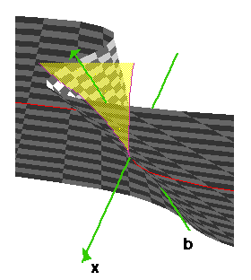
Fig. 4. The projection (transparent yellow) of the fold proper (the pleat, the Whitney-pleat) on (a,b) space is called the cusp-catastrophe or the Riemann-Huguenot-catastrophe. The edge of the cusp, the bifurcation set, is shown in violet colour, the projection of the a-axis on the fold in red colour, this curve is the organizing centre of the fold, y = x3. Remember that the system has four dimensions; what is shown here is only the graph of the derivative. Each single point of the sheet represents a potential curve (types in Fig. 3), slightly differing from its neighbours.
Calculating the cusp
Zeeman (1977) has treated stock exchange and currency behaviour from one and the same model, namely what he terms the cusp catastrophe with a slow feedback. Here the rate of change of indexes (or currencies) is considered as dependent variable, while different buying patterns ("fundamental" /N in fig. 5/ and "chartist" /S in fig. 5/) serve as normal and splitting parameters. Zeeman argues: the response time of X to changes in N and S is much faster than the feedback of X on N and S, so the flow lines will be almost vertical everywhere. If we fix N and S, X will seek a stable equilibrium position, an attractor surface (or: two attractor surfaces, separated by a repellor sheet and "connected" by catastrophes; one sheet is inflation/bull market, one sheet deflation/bear market, one catastrophe collapse of market or currency. Note that the second catastrophe is absent with the given flow direction. This is important, it tells us that the whole pattern can be manipulated, "adapted" by means of feedbacks/flow directions). Close to the attractor surface, N and S become increasingly important; there will be two horizontal components, representing the (slow) feedback effects of N and S on X. The whole sheet (the fold) is given by the equation X3 - (S - So)X - N = 0, the edge of the cusp by 3X2 + So = S, which gives the equation 4(S - So)3 = 27 N2 for the bifurcation curve. The model is shown in Fig. 5.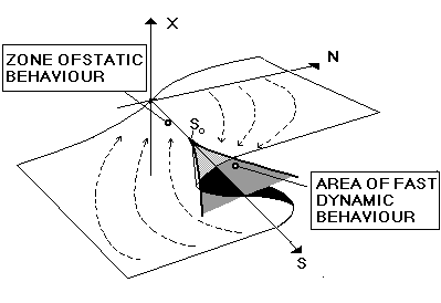
Fig. 5. "Cusp with a slow feedback", according to Zeeman (1977). X, the state variable, measures the rate of change of an index, N = normal parameter, S = splitting parameter, the catastrophic behaviour begins at So. On the back part of the upper sheet, N is assumed constant and dS/dt positive, on the fore part dN/dT is assumed to be negative and dS/dt positive; this gives the flow direction of the feedback. On the fore part of the lower sheet both dN/dt and dS/dt are assumed to be negative, on the back part dN/dt is assumed to be positive and dS/dt still negative, this gives the flow direction of feedback on this sheet. The cusp projection on the {N,S}-plane is shaded grey, the visible part of the repellor sheet black. (The reductionist character of these models must always be kept in mind; here two obvious key parameters are considered, while others of a weaker or more ephemeral kind - e.g. interest levels - are ignored.)
TO BE CONTINUED
LITERATURE
- Stjernfelt, F. (1992): Formens betydning. Katastrofeteori og semiotik. Akademisk forlag. In Danish, with semiotics as main subject field, written by the foremost introducer of the catastrophe theory in Scandinavia; this book was my first really helpful introduction to catastrophe theory after reading Thom (2). The proofreading of the text is catastrophic; it could be said in its favour that it tests the attention of the reader.
- Thom, R. (1971): Topological models in biology. In: Towards a Theoretical Biology, ed. C. H. Waddington. Four volumes: 1969 (Prolegomena), 1970 (Drafts), 1971 (Sketches), 1972 (?). This is a wonderful project, with utopian overtones; a couple of texts are among the most valuable biological papers (or: "meta"-papers) written in the 20th century.
- Zeeman, E. C. (1977): Catastrophe Theory. Selected Papers 1972 - 1977. Addison-Wesley Publ. Co. This book is a patchwork: a collection of lecture scripts and papers, but still very illuminating. Zeeman has a typically British inclination towards empiricism, 'positive' thought, always grabbing for any possible application; throughout the book he tries to reconcile this attitude with the more esoteric, lofty approach of Thom, the result being a highly creative culture clash between "English" and "French" basic attitudes to thinking. (On the other hand Thom's "Songeries ferroviaires" from 1979 seems to be British-inspired; this fruitful exchange has never been unilateral). In this way the book also comes to depict the practical difficulties of the catastrophe theory ("Where are the damn morphogens?") as much as its possibilities.
- Poston, T. & I. Stewart (1978): Catastrophe Theory and its Applications. Pitman Publishers. A more strict textbook with all the mathematics one can need and use, dedicated to E. C. Zeeman, but the authors also acknowledge: "In the beginning was Thom." This book is extremely rewarding reading, function theory should be taught this way! I particularly noted the following lines in the preface: It has been said more than once that it is possible to apply Thom's theorem without understanding the mathematics behind it: we disagree. In fact we disagree with the implication that it is Thom's theorem that should be applied: analysis of the most solid and successful applications shows that the methods and concepts that lie behind the theorem are often of greater importance than the result itself. (My bold type; CP). I am inclined to agree - but in the long run most applications are dead without the metaphysical "spark" from Thom! The optimal approach in these matters is bimodal, at least in this respect.
- Rosen, R. (1970): Dynamical System Theory in Biology. Vol. 1: Stability Theory and its Applications. John Wiley and Sons. The name Rosen is still among the first to come up when the question is put: Who understands e. g. structural stability - more than the "inner circle" of catastrophe theory? The early year of publication indicates, that Robert Rosen should be included among the pioneers of at least stability theory. I haven't read much yet, but to my delight I understand what I didn't understand when I opened the book twenty years ago. There is still hope for us: the human mind can be improved.
- An "engineering", practical approach - in the tradition of Thom and Zeeman, who did similar things - to catastrophe theory can be found on http://perso.wanadoo.fr/l.d.v.dujardin/ct, "An introduction to Catastrophe Theory for experimentalists" by Lucien Dujardin, Laboratory of Parasitology, University of Lille. I love labyrinthic web structures of this kind, with small surprises behind every new corner. Anyone who wants to feel his or her way to catastrophe theory by means of the computer keyboard should visit this page. One French, one English version, I will return with more comment when I have read it all. [CP]
(This excurse has been spotted by readers from the first second - the effectivity of search engines always amazes me! It is my first attempt with catastrophe theory, so there will be initial errors, in language, in thinking. I will detect them in due time - but any suggestion saving me from a blunder will be welcome! / Christer Persson)